Control of Three Link Acrobot

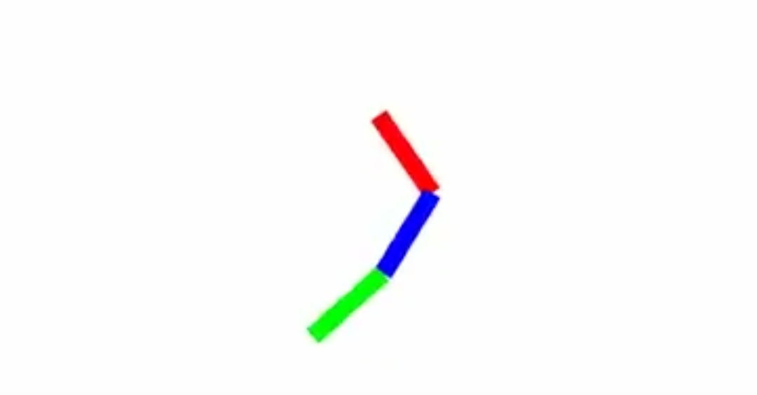
MAE454: Optimal Control of Non-Linear Systems

Link to Project Report and Mathematica Code.

Project Details

An Acrobot is usually described as a two-link pendulum, where the first link is passive and the second link can be actively controlled. There have been many papers and videos about controlling the acrobot to swing to an upright position.

For my MAE454 project, I decided to try to control and simulate a three-link acrobot. Similar to the two-link acrobot, the first link is passive while the second and third link are actively controlled. The acrobot will start in the hanging position, and will try to swing itself to an upright position.

The Lagrangian (L) and the Euler-Lagrange equations were used to solve for the dynamics of the system. The effects of rotational inertia were also accounted for; implementation of this can be found in the Mathematica code.

The pseudocode of the iterative optimal control algorithm used to find the optimal control is described below:

\begin{equation} \bar{\xi_0} \in \mathcal{L} \text{ or } \xi_0 \in \mathscr{T}, \hspace{12cm} (1) \hspace{24cm} \end{equation}

\begin{equation} J(\bar{\xi}), \hspace{14.2cm} (2) \hspace{24cm} \end{equation}

\begin{equation} \alpha \in (0, \frac 12), \hspace{13.2cm} (3) \hspace{24cm} \end{equation}

\begin{equation} \beta \in (0, 1), \hspace{13.4cm} (4) \hspace{24cm} \end{equation}

\begin{equation} \text{and } \epsilon \text{ (a small number)} \hspace{11.04cm} (5) \hspace{24cm} \end{equation}

\begin{equation} \textbf{while } \Vert \zeta_i-1 \Vert \gt \epsilon \textbf{ do} \hspace{11.2cm} (6) \hspace{24cm} \end{equation}

\begin{equation} \text{compute descent direction: } \hspace{8cm} \tag{7} \end{equation}

\begin{equation} \zeta_i = \underset{\zeta\in\mathcal{T}, \mathscr{P}(\bar{\xi}) \in \mathscr{T}}{\arg\min} DJ(\mathscr{P}(\bar{\xi_i})) \circ D\mathscr{P}(\bar{\xi_i}) \circ \bar{\zeta} + \frac 12 \Vert\zeta\Vert^2 \hspace{4cm} \tag{8} \end{equation}

\begin{equation} \text{compute line search using descent direction } \zeta_i: \hspace{4.5cm} \tag{9} \end{equation}

\begin{equation} n = 0; \hspace{12cm} \tag{10} \end{equation}

\begin{equation} \textbf{while } J(\mathscr{P}(\bar{\xi_i} + \gamma\zeta_i)) \gt J(\mathscr{P}(\bar{\xi_i})) + \alpha\gamma DJ(\mathscr{P}(\bar{\xi_i})) \circ D\mathscr{P}(\bar{\xi_i}) \circ \bar{\zeta}\textbf{ do} \hspace{.5cm} \tag{11} \end{equation}

\begin{equation} n = n + 1; \hspace{8cm} \tag{12} \end{equation}

\begin{equation} \gamma = \beta^n; \hspace{8.5cm} \tag{13} \end{equation}

\begin{equation} \textbf{end} \hspace{12.5cm} \tag{14} \end{equation}

\begin{equation} \xi_{i+1} = \mathscr{P}(\bar{\xi_i} + \gamma\zeta_i); \hspace{9.5cm} \tag{15} \end{equation}

\begin{equation} i = i + 1; \hspace{11.5cm} \tag{16} \end{equation}

\begin{equation} \textbf{end} \hspace{14.3cm} (17) \hspace{24cm} \end{equation}

where the cost function is defined as:

\begin{equation} J = \int_0^\mathcal{T} \frac 12 (x-x_d)^TQ(x-x_d) + \frac 12 (u-u_d)^TR(u-u_d) dt + \frac 12 ((x(\mathcal{T})-x_d(\mathcal{T}))^TP_1(x(\mathcal{T})-x_d(\mathcal{T})) \end{equation}

What Does the Algorithm Mean?

The variables of the cost function $J$:

• $\mathcal{T}$: Desired final time.
• $x_d$: Desired state trajectory.
• $u_d$: Desired control trajectory.
• $x_d(\mathcal{T})$: Desired end state at final time.
• $u_d(\mathcal{T})$: Desired control state at final time.
• $Q$: Square diagonal matrix parameter used to determine how much the state should affect the cost value. The larger Q is, the more we want the system to follow the desired trajectory. The smaller Q is, the less we care about the system following the desired trajectory.
• $R$: Square diagonal matrix parameter used to determine how much control input is desired in the system. The larger R is, the smaller we want control to be put into the system. The smaller R is, the less we care about how much input we put into the system.
• $P_1$: Square diagonal matrix parameter used to determine how important it is to reach the final desired goal. The larger $P_1$ is, the more we want the system to reach the desired end goal. The smaller $P_1$ is, the less we care about the system reaching the end goal.

Q, R, and $P_1$ are parameters that can be tuned to find an ideal solution.

Lines 1 - 5 are the initial conditions of the system. Variable definitions are defined below.

• $\bar{\xi_0}$ : Defined as a curve ,$(\bar{x_0}, \bar{u_0})$, where $\bar{x_0}$ is the state of the system and $\bar{u_0}$ is the control required to reach the desired goal. $\bar{\xi_0}$ can potentially be dynamically infeasible.
• $\xi_0$ : Defined as a trajectory , $(x_0, u_0)$, where $x_0$ is the state of the system and $u_0$ is the control required to reach the desired goal. $\xi_0$ is dynamically feasible.
• $\mathcal{L}$: The set of all trajectories
• $\mathscr{T}$: The set of all feasible trajectories.
• $\alpha$ and $\beta$: Parameters to find the ideal step size in the descent direction (Armijo Line Search Algorithm). Typical values of $\alpha$ and $\beta$ are .4 and .7, respectively.
• $\epsilon$: Algorithm terminating condition

Other useful variable definitions:

• $\zeta$: Descent direction
• $\mathscr{P}$: Projection function that projects onto a dynamically feasible trajectory.
• $D$: Take the derivative of the next function.
• $\gamma$: Step size to take in the descent direction.

Line 7-8 describes the method to find the descent direction. The descent direction describes the direction the minimum of the trajectory is located in.

Line 10-14 describes the method to the step size to take in the descent direction. This method is also known as the Armijo Line Search.

Line 15-16 describes the update to the the new desired trajectory. The new error value that can be checked on the outer while loop can be calculated by taking the norm of the derivative of the cost function of the updated trajectory.

Ideal Solution